Generated with Stable Diffusion - prompt "ecg electrodes on human body abstract"

Table of contents

• Introduction

• What is a Butterworth filter?

  • Theory
  • Example

• How to code a Butterworth filter in C++

  • From frequency to time domain
  • C++ implementation
  • Full C++ code

• How to test your filter with Python

  • Step by step guide
  • Full Python Code
  • Automating the Build and Test Process
• Conclusion

Introduction

Biomedical signals are crucial for healthcare but are often distorted by noise. One way to clean up these signals is through filtering. In this tutorial, I'll show you how to design a Butterworth filter using C++ and then test it using Python.

I'll cover:

1. What Butterworth filters are and why they're useful.
2. How to code one in C++.
3. How to test your filter with Python by simulating biomedical signals.

By the end of this guide, you'll know how to create and test a Butterworth filter for cleaner biomedical signals. Let's dive in!

What is a Butterworth filter?

Theory

A Butterworth filter is like a sieve for your biomedical signals. Imagine you have a mix of useful information and unwanted noise. This filter helps you keep the useful parts and get rid of the noise, making the signal clearer. It's popular because it keeps the good stuff almost unchanged while effectively removing the bad stuff. You can adjust its strength and where it starts filtering to fit your specific needs.

The Butterworth filter is characterized by its frequency response equation:

Where:

• $f$ is the frequency of the input signal
• $f_c$ is the cutoff frequency, the point where the filter starts to work. Frequencies below this value are mostly kept, and frequencies above are reduced
• $n$ is the order of the filter. A higher number here makes the filter remove the unwanted frequencies more sharply
• $H(f)$ is the frequency response of the filter. It shows how strong the filter is at a particular frequency $f$. If $H(f)$ is close to 1, the filter lets that part of the signal pass through almost unchanged

Example

Imagine you have a Butterworth filter with a cutoff frequency ($f_c$) of 10 Hz and an order $n$ of 2. If you apply it to a signal with a frequency of 5 Hz, the filter will let it pass almost unchanged. But if the signal has a frequency of 20 Hz, the filter will reduce it significantly.

Let's put these numbers into the equation to see what we get.

We can take a look at the frequency response of this filter to see how it works. The graph below shows the frequency response of a Butterworth filter with a cutoff frequency of 10 Hz and an order of 2.

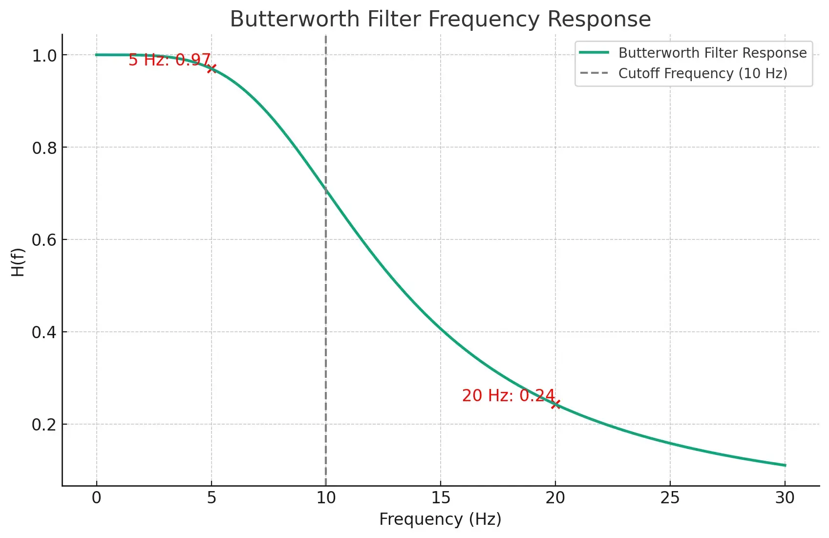
As you can see, the filter lets frequencies below 10 Hz pass almost unchanged. But it reduces frequencies above 10 Hz more and more as they get higher. This is what makes the filter so useful for cleaning up biomedical signals. It keeps the useful parts of the signal almost unchanged while reducing the noise.

Lets take a look at the input signal and the filtered signal to see how the filter works in practice.

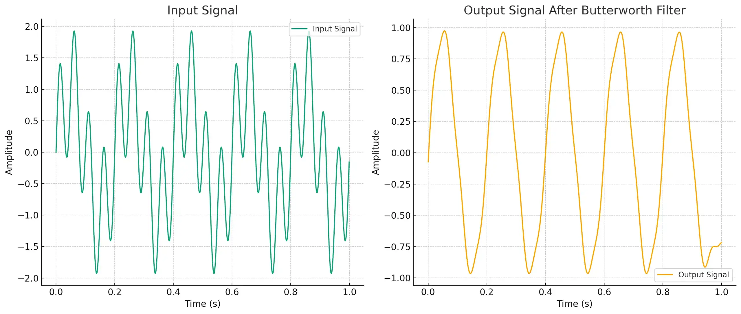
• Input Signal: The first graph shows a signal that's a mix of a 5 Hz sine wave and a 20 Hz sine wave. You can see that it looks a bit messy because of the two different frequencies combined.
• Output Signal After Butterworth Filter: The second graph shows what happens after we pass the input signal through the Butterworth filter. The 20 Hz component is mostly removed, leaving us with a cleaner, primarily 5 Hz sine wave.

How to code a Butterworth filter in C++

From frequency to time domain

The Butterworth filter is often defined in the frequency domain using its frequency response equation $H(f)$. However, in practical applications, especially in digital signal processing, it's implemented using a time-domain difference equation. This equation is a bit more complicated, but it's easier to implement in code.

$H(s)$ is the Laplace transform of the second-order Butterworth filter:

We can convert this to a difference equation using the bilinear transform:

Where:

• $T$ is the sampling period
• $z$ is the complex variable in the z-plane
• $s$ is the complex variable in the s-plane
• $H(s)$ is the Laplace transform of the second-order Butterworth filter

After applying the bilinear transform, we get the following difference equation:

Let us introduce the normalized angular frequency $\omega$. It is used to calculate the coefficients of the difference equation. We can calculate it using the following formula:

Where:

• $f_c$ is the cutoff frequency
• $f_s$ is the sampling frequency

Sampling frequency is the number of samples per second. It's the rate at which we measure the signal. For example, if we measure a signal at 100 Hz, we get 100 samples per second. If we measure it at 1000 Hz, we get 1000 samples per second.

Let us also introduce the scaling factor $c$ used to normalize the coefficients of the digital filter. We can calculate it using the following formula:

C++ implementation

1. Calculate $\omega$ and $c$ using the formulas above.

double omega = tan(M_PI * fc / fs);
double c = 1.0 / (1.0 + sqrt(2.0) * omega + omega * omega);

2. Calculate the coefficients of the difference equation.

double a1 = 2.0 * (omega * omega - 1.0) * c;
double a2 = (1.0 - sqrt(2.0) * omega + omega * omega) * c;

double b0 = omega * omega * c;
double b1 = 2.0 * b0;
double b2 = b0;

3. Filtering the signal.

double output = b0 * input + b1 * x_prev[0] + b2 * x_prev[1] - a1 * y_prev[0] - a2 * y_prev[1];

4. Update the previous values.

x_prev[1] = x_prev[0];
x_prev[0] = input;

y_prev[1] = y_prev[0];
y_prev[0] = output;

Full C++ code

Here's the full C++ code for the Butterworth filter. It's a class that you can use in your own projects. It also has a C interface for testing with Python.

#ifndef BUTTERWORTH_FILTER_H
#define BUTTERWORTH_FILTER_H

class ButterworthFilter {
private:
    double x_prev[2];
    double y_prev[2];
    double cutoffFrequency;
    double sampleRate;

public:
    ButterworthFilter(double cutoffFreq, double sampleRate);
    double filter(double input);
};

#endif // BUTTERWORTH_FILTER_H

#include <iostream>
#include <cmath>

class ButterworthFilter {
private:
    double x_prev[2];
    double y_prev[2];
    double cutoffFrequency;
    double sampleRate;

public:
    ButterworthFilter(double cutoffFreq, double sampleRate) {
        x_prev[0] = 0.0;
        x_prev[1] = 0.0;
        y_prev[0] = 0.0;
        y_prev[1] = 0.0;

        this->cutoffFrequency = cutoffFreq;
        this->sampleRate = sampleRate;
    }

    double filter(double input) {
        double omega = tan(M_PI * cutoffFrequency / sampleRate);
        double c = 1.0 / (1.0 + sqrt(2.0) * omega + omega * omega);

        double a0 = 1.0;
        double a1 = 2.0 * (omega * omega - 1.0) * c;
        double a2 = (1.0 - sqrt(2.0) * omega + omega * omega) * c;

        double b0 = omega * omega * c;
        double b1 = 2.0 * b0;
        double b2 = b0;

        double output = b0 * input + b1 * x_prev[0] + b2 * x_prev[1] - a1 * y_prev[0] - a2 * y_prev[1];

        x_prev[1] = x_prev[0];
        x_prev[0] = input;

        y_prev[1] = y_prev[0];
        y_prev[0] = output;

        return output;
    }
};

// C interface for testing with Python
extern "C" {
    ButterworthFilter* ButterworthFilter_new(double cutoffFreq, double sampleRate) {
        return new ButterworthFilter(cutoffFreq, sampleRate);
    }

    double ButterworthFilter_filter(ButterworthFilter* filter, double input) {
        return filter->filter(input);
    }

    void ButterworthFilter_delete(ButterworthFilter* filter) {
        delete filter;
    }
}

We can build this code into a shared library using the following command:

g++ -shared -o ButterworthFilter.so -fPIC ButterworthFilter.cpp

• -shared tells the compiler to create a shared library
• -o ButterworthFilter.so tells the compiler to name the output file ButterworthFilter.so
• -fPIC tells the compiler to create position-independent code. This is required for shared libraries

How to test your filter with Python

Step by step guide

1. Import Libraries

import ctypes
import numpy as np
import matplotlib.pyplot as plt
import wfdb

• ctypes is a Python library for calling C functions. We'll use it to call the C++ code we wrote earlier.
• numpy is a Python library for scientific computing. We'll use it to generate the input signal.
• matplotlib is a Python library for plotting graphs. We'll use it to plot the input and output signals.
• wfdb is library for reading, writing, and processing physiological signals like ECGs in formats used by PhysioNet. It provides tools for signal visualization, basic signal processing, and interaction with PhysioNet databases.

1. Load the C++ library

lib = ctypes.cdll.LoadLibrary('./ButterworthFilter.so')

3. Define Python Class for C Struct

class ButterworthFilter(ctypes.Structure):
    _fields_ = []

Creates an empty Python class that will correspond to the C ButterworthFilter struct.

4. Define Function Prototypes

lib.ButterworthFilter_new.argtypes = [ctypes.c_double, ctypes.c_double]
lib.ButterworthFilter_new.restype = ctypes.POINTER(ButterworthFilter)

lib.ButterworthFilter_filter.argtypes = [ctypes.POINTER(ButterworthFilter), ctypes.c_double]
lib.ButterworthFilter_filter.restype = ctypes.c_double

lib.ButterworthFilter_delete.argtypes = [ctypes.POINTER(ButterworthFilter)]

Sets the argument types and return types for the C functions. This ensures that Python and C understand each other.

5. Load ECG Signal

record = wfdb.rdrecord('sample-data/100', channels=[0], sampfrom=0, sampto=1500)
ecg_signal = record.p_signal.flatten()

Reads an ECG signal from the file 'sample-data/100' using the wfdb package. Flattens it to a one-dimensional array.

6. Create an Instance of the Filter

cutoff_frequency = 35.0
sample_rate = 360.0

filter_instance = lib.ButterworthFilter_new(cutoff_frequency, sample_rate)

7. Filter the ECG Signal

filtered_ecg_signal = np.zeros_like(ecg_signal)
for i in range(len(ecg_signal)):
    filtered_ecg_signal[i] = lib.ButterworthFilter_filter(filter_instance, ecg_signal[i])

8. Clean Up

lib.ButterworthFilter_delete(filter_instance)

Deletes the filter instance to free up memory.

9. Plot the Input and Output Signals

fig, (ax1, ax2) = plt.subplots(2, 1, sharex=True)
fig.suptitle('ECG signal before and after filtering')
ax1.plot(ecg_signal)
ax1.set_ylabel('Voltage (mV)')
ax1.grid()
ax2.plot(filtered_ecg_signal)
ax2.set_xlabel('Time (ms)')
ax2.set_ylabel('Voltage (mV)')
ax2.grid()
plt.show()

Full Python Code

Here's the full Python code for testing the Butterworth filter. It's a script that you can run to see the results.

import ctypes
import numpy as np
import matplotlib.pyplot as plt

# Load the wfdb package
import wfdb

# Load the shared library
lib = ctypes.CDLL('./ButterworthFilter.so')

# Create an instance of the ButterworthFilter class
class ButterworthFilter(ctypes.Structure):
    _fields_ = []

# Define the ButterworthFilter constructor prototype
lib.ButterworthFilter_new.argtypes = [ctypes.c_double, ctypes.c_double]
lib.ButterworthFilter_new.restype = ctypes.POINTER(ButterworthFilter)

# Define the filter function prototype
lib.ButterworthFilter_filter.argtypes = [ctypes.POINTER(ButterworthFilter), ctypes.c_double]
lib.ButterworthFilter_filter.restype = ctypes.c_double

# Define the delete function prototype
lib.ButterworthFilter_delete.argtypes = [ctypes.POINTER(ButterworthFilter)]

# Load ECG signal using the wfdb package
record = wfdb.rdrecord('sample-data/100', channels=[0], sampfrom=0, sampto=1500)
ecg_signal = record.p_signal.flatten()

# Create an instance of ButterworthFilter
cutoff_frequency = 35.0
sample_rate = 360.0

filter_instance = lib.ButterworthFilter_new(cutoff_frequency, sample_rate)

# Filter the ECG signal using your ButterworthFilter class
filtered_ecg_signal = np.zeros_like(ecg_signal)
for i in range(len(ecg_signal)):
    filtered_ecg_signal[i] = lib.ButterworthFilter_filter(filter_instance, ecg_signal[i])

# Clean up
lib.ButterworthFilter_delete(filter_instance)

# Create two separate plots
fig, (ax1, ax2) = plt.subplots(2, 1, sharex=True)
fig.suptitle('ECG signal before and after filtering')

# Plot the original ECG signal
ax1.plot(ecg_signal)
ax1.set_ylabel('Voltage (mV)')
ax1.grid()

# Plot the filtered ECG signal
ax2.plot(filtered_ecg_signal)
ax2.set_xlabel('Time (ms)')
ax2.set_ylabel('Voltage (mV)')
ax2.grid()

plt.show()

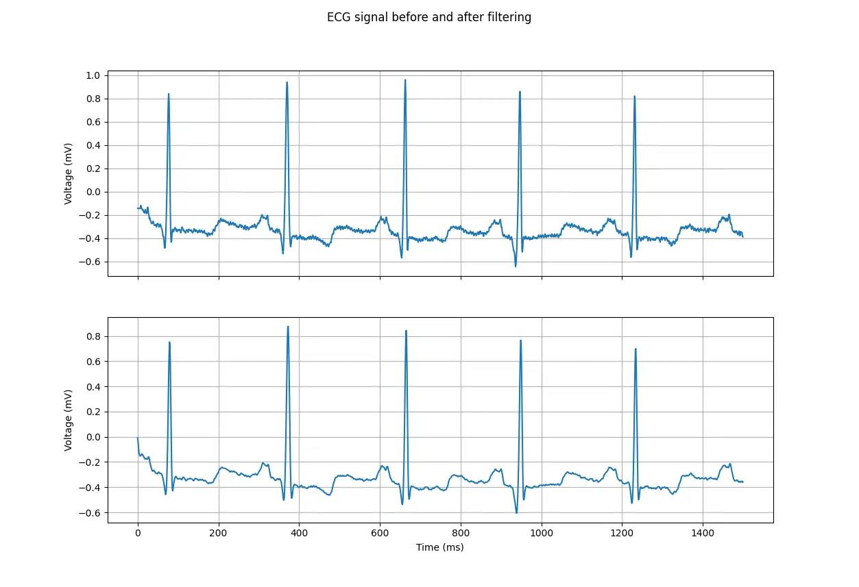
ECG signal before and after filtering

As we can see, the filter removes the high-frequency noise from the ECG signal, leaving us with a much cleaner signal.

Automating the Build and Test Process

We can automate the build and test process using a simple python script. It will build the C++ code into a shared library and then run the Python script to test it.

import os
import subprocess

# Build the C++ shared library
build_command = "g++ -shared -o ButterworthFilter.so -fPIC ButterworthFilter.cpp"

try:
    subprocess.run(build_command, shell=True, check=True)
    print("C++ shared library built successfully.")
except subprocess.CalledProcessError:
    print("Error building the C++ shared library.")
    exit(1)

# Test the library using Python
test_command = "python3 test_library.py"

try:
    subprocess.run(test_command, shell=True, check=True)
except subprocess.CalledProcessError:
    print("Error testing the C++ shared library with Python.")
    exit(1)

Conclusion

This tutorial provided a step-by-step guide on how to design, implement, and test a Butterworth filter for biomedical signal processing. We used C++ for the heavy lifting of filter design due to its performance advantages, making it ideal for real-time applications. Python was used for the testing phase, leveraging its rich ecosystem of scientific libraries for easy and effective validation.